There are many tutorials on neural networks and deep learning, that use the handwritten digits data set (MNIST) to show what deep learning can give you. It generally trains a model to recognize the digits and show it’s better than a logistic regression. Many such tutorials also say something about auto-encoders and how they should be able to pre-process images, for example to get rid of noise and improve recognition on noisy (and hence more realistic?) images. Rarely, though, is that worked out into any amount of detail.
This blog post is a short summary, and a full version with code and output is available at my github. Lazy me has taken some shortcuts: I have pretty much always used default values of all models I trained, I have not investigated how they can be improved by tweaking (hyper-)parameters and I have only used simple dense networks (while convolutional neural nets might be a very good choice for improvement in this application). In some sense, the model can only get better in a realistic setting. I have compared to simple but popular other models, and sometimes that comparison isn’t very fair: the training time of the (deep) neural network models often is much longer. It is nevertheless not very easy to define a “fair comparison”. That said, going just that little bit beyond the recognition of the handwritten set can be done as follows.
The usual first steps
To start off, the data set of MNIST has a whole bunch of handwritten digits, a random sample of which looks like this:
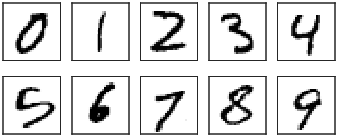
The images are 28×28 pixels and every pixel has a value ranging from 0 to 255. All these 784 pixel values can be thought of as features of every image, and the corresponding labels of the images are the digits 0-9. As such machine learning models can be trained, to categorize the images into 10 categories, corresponding to the labels, based on 784 input variables. The labels in the data set are given.
Logistic regression can do this fairly well, and get roughly 92% of the labels right on images it has not seen while training the model (an independent test set), after being trained on about 50k such images. A neural network with one hidden layer (of 100 neurons, the default of the multi-layer perceptron model in scikit-learn) will get about 97.5% right, a significant improvement to the simple logistic regression. The same model with 3 hidden layers of 500, 200 and 50 neurons respectively will further improve that to 98%. When similar models are implemented in Tensorflow/Keras, with proper activation functions, will get about the same score. So far, so good, and this stuff is in basically every tutorial you have seen.
Let’s get beyond that!
Auto-encoders and bottleneck networks
Auto-encoders are neural networks that typically use many input features, then go through a narrower hidden layer and then as output reproduce the input features. Graphically, it would look like this, with the output being identical to the input:
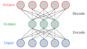
This means that, if the network performs well (i.e. if the input is reasonably well reproduced), all information about the images is stored into a smaller number of features (equal to the number of neurons in the narrowest hidden layer), which can be used as compression technique for example. It turns out that this also works very well to recover images from noisy variants of the images (the idea being that the network figures out the important bits, i.e. the actual image, from the unimportant, i.e. the noise pixels).
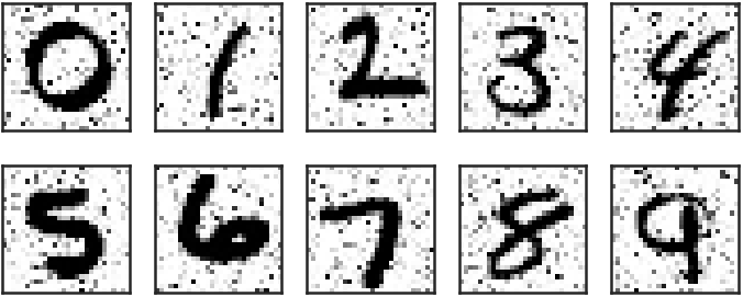
I created a set of noisy MNIST images looking, for 10 random examples, like this:
A simple auto-encoder, with hidden layers of 784, 256, 128, 256 and 784 neurons (note the symmetry around the bottleneck layer!), respectively does a fair job at reproducing noise-free images:
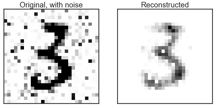
It’s not perfect, but it is clear that the “3” is much cleaner than it was before “de-noising”. A little comparison of recognizing the digits on noisy versus de-noised images shows that it pays to do such a pre-processing step before: the model trained on the clean images only recovers 89% of the correct labels on the noisy images, but 94% after de-noising (a factor 2 reduction in the number of wrongly identified labels). Note that all of this is done without any optimization of the model. The Kaggle competition page on this data set shows many optimized models and their amazing performance!
Dimension reduction and visualization
To investigate whether any structure exists in the data set of 784 pixels per image, people often, for good reasons, resort to manifold learning algorithms like t-SNE. Such algorithm go from 784 dimensions to, for example, 2, thereby keeping local structure intact as much as possible. A full explanation of such algorithms goes beyond the scope of this post, I will just show the result of it here. The 784 pixels are reduced to two dimensions and in this figure I plot those two dimensions against each other, color coded by the image label (so every dot is one image in the data set):
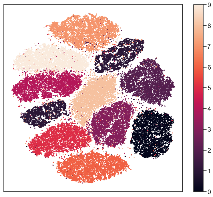
The labels seem very well separated, suggesting that reduction of dimensions can go as far as down to two dimensions, still keeping all the information to recover the labels to reasonable precision. This inspired me to try the same with a simple deep neural network. I go through a bottleneck layers of 2 neurons, surrounded by two layers of 100 neurons. Between the input and that there is another layer of 500 neurons and the output layer obvioulsy has 10 neurons. Note that this is not an auto-encoder: the output are the 10 labels, not the 784 input pixels. That network recovers more than 96% of the labels correctly! The output of the bottleneck layer can be visualized in much the same way as the t-SNE output:
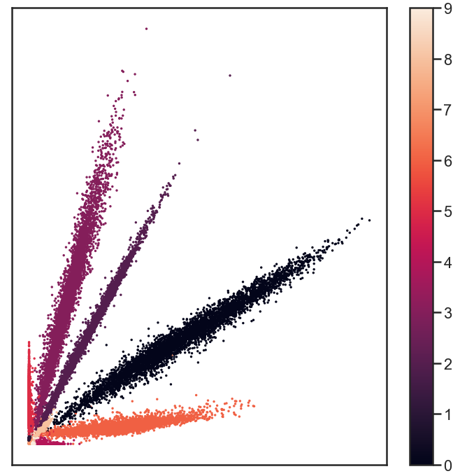
It looks very different from the t-SNE results, but upon careful examination, there are similarities in terms if which digits are more closely together than others, for example. Again, this distinction is good enough to recover 96% of the labels! All that needs to be stored about images is 2 numbers, obtained from the encoding part of the bottleneck network, and using the decoding bit of the network, the labels can be recovered very well. Amazing, isn’t it?
Outlook
I hope I have shown you that there are a few simple steps beyond most tutorials that suddenly make these whole deep neural network exercises seem just a little bit more useful and practical. Are there applications of such networks that you would like to see worked out in some detail as well? Let me know, and I just might expand the notebook on github!
One thought on “Beyond the recognition of handwritten digits”