blog posts – Marcel Haas – Data, Science & More

What determines what I teach?

I very recently quit a teaching program that I have been part of for more than four years, to which I had a personal connection after all those years. Besides it being lucrative, it was also a program that was for a good part shaped by me and colleagues and which was fun and fulfilling to teach. Why quit, you might ask.

The program, consisting of modules for data scientists, analytics translators and managers/executives, was a collaboration between a consulting company, Ortec, and the Amsterdam Business School, a department of the University of Amsterdam that organizes a lot of executive education. The data scientist program was ruthlessly killed about a year ago, because of fierce competition from online platforms. Face-to-face education is more effective and in my opinion worthwhile, but if you can’t offer the right program for the right price, then it isn’t weird to decide not to. That so many people think you can learn such skills through watching a few videos and typing in two lines of code in a automatically checking code interpreter continues to amaze me and I bet we will see the devastating effects of this, now still junior, generation of Youtube data scientists in due time. But I digress.

The module for analytics translators is still alive and just these past few months I have still been teaching it. Fulfilling as always, I spent two half days in lecture rooms in hotels with a group of enthusiastic participants. The program this time was already rather different from what it had been before, and with the feedback of the current cohort, leadership decided to do another round of modifications.

Do not misunderstand me: continuously updating your educational offerings is what a good teacher does. Incorporating feedback from participants (or students) is crucial, as only they can properly judge whether your efforts help them reach their learning goals. One quote of the program director in the process made me scratch my head though:

I am just trying to design a program that I can sell.

Sure, selling your program is important, as otherwise there is no program. I get that. And for consulting companies (this program director is not with the consulting party in the collaboration) this may be the most or even only viable way of running business. I think, though, that people come to trusted educational institutions like universities for a different reason. A university does not design a curriculum for sales. It sets learning goals (which may well be (job-) market informed!) and then designs an educational pathway to best reach those goals. What people need to learn is determined by where they want to end up, not by what is a sexy set of courses that happens to be easily marketed.

Teachers are teaching what they teach for two reasons. Firstly, they want to convey knowledge and skills that they have to students who want to learn. They think about the right educational means to help the students gain the knowledge and master the skills. Secondly, they are specialists in the field in which they teach, which means that they understand like no other what is necessary to learn, before one can become a specialist in that field, too. Few astronomers truly enjoy the first-year linear algebra they need to master and rarely do psychologist enjoy their statistics classes in undergrad, but these happen to be crucial ingredients to grow into the field that you want to be part of.

Besides the communication between the various people in this program detoriating to levels that I didn’t want to accept anymore, the fact that the curriculum went from specialist-informed to marketing and sales opportunity informed was the straw that broke the camel’s back. I want to be a proud teacher. Proud teachers design a program that is the best they can do to help students reach meaningful goals. You are very welcome to set learning goals based on all kinds of arguments, including sales, but once the learning goals are set, you should trust the professional’s teaching experience to manufacture a great, fun, and helpful course or program. It will be better for everyone’s motivation.

PS. More on my new academic role soon, presumably!

Proper statistics is Bayesian

I was already convinced years ago, by videos and a series of blog posts by Jake VanderPlas (links below), that if you do inference, you do it the bayesian way. What am I talking about? Here is a simple example: we have a data set with x and y values and are interested in their linear relationship: y = a x + b. The numbers a and b will tell us something we’re interested in, so we want to learn their values from our data set. This is called inference. This linear relationship is a model, often a simplification of reality.

The way to do this you learn in (most) school(s) is to make a Maximum Likelihood estimate, for example through Ordinary Least Squares. That is a frequentist method, which means that probabilities are interpreted as the limit of the relative frequencies for very many trials. Confidence intervals are the intervals that describe where the data would lie after many repetitions of the experiment, given your model.

In practice, your data is what it is, and you’re unlikely to repeat your experiment many times. What you are after is an interpretation of probability that describes the belief you have in your model and its parameters. That is exactly what Bayesian statistics gives you: the probability of your model, given your data.

For basically all situations in science and data science, the Bayesian interpretation of probability is what suits your needs.

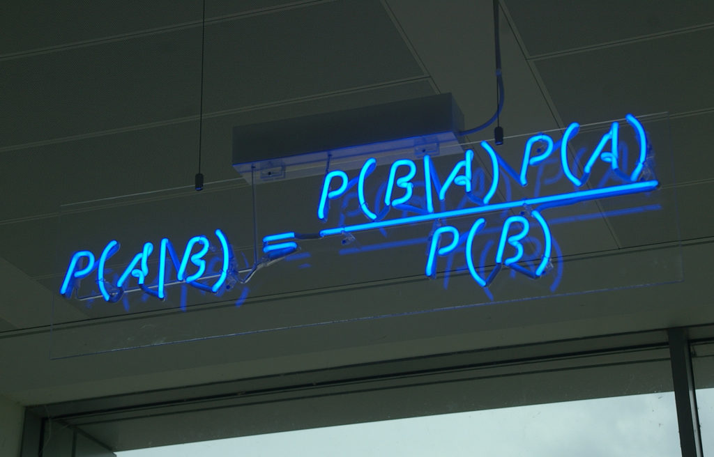
What, in practice, is the difference between the two? All of this is based on Bayes’ theorem, which is a pretty basic theorem following from conditional probability. Without all the interpretation business, it is a very basic result, that no one doubts and about which there is no discussion. Here it is:

Now replace A by “my model (parameters)” and B by “the data” and the difference between inference in the frequentist vs Bayesian way shines through. The Maximum Likelihood estimates P(data | model), while the bayesian posterior (the left side of the equation) estimates P (model | data), which arguably is what you should be after.

As is obvious, the term that makes the difference is P(A) / P(B), which is where the magic happens. The probability of the model is hat is called the prior: stuff we knew about our model (parameters) before our data came in. In a sense, we knew something about the model parameters (even if we knew very very little) and update that knowledge with our data, using the likelihood P(B|A). The normalizing factor P(data) is a constant for your data set and for now we will just say that it normalizes the likelihood and the prior to result in a proper probability density function for the posterior.

The posterior describes the belief in our model, after updating prior knowledge with new data.

The likelihood is often a fairly tractable analytical function and finding it’s maximum can either be done analytically or numerically. The posterior, being a combination of the likelihood and the prior distribution functions can quickly become a very complicated function that you don’t even know the functional form of. Therefore, we need to rely on numerical sampling methods to fully specify the posterior probability density (i.e. to get a description of how well we can constrain our model parameters with our data): We sample from the priors, calculate the likelihood for those model parameters and as such estimate the posterior for that set of model parameters. Then we pick a new point in the priors for our model parameters, calculate the likelihood and then the posterior again and see if that gets us in the right direction (higher posterior probability). We might discard the new choice as well. We keep on sampling, in what is called Markov Chain Monte Carlo process in order to fully sample the posterior probability density function.

On my github, there is a notebook showing how to do a simple linear regression the Bayesian way, using PyMC3. I also compare it to the frequentist methods with stasmodels and scikit-learn. Even in this simple example, a nice advantage of getting the full posterior probability density shines: there is an anti-correlation between the values for slope and intercept that makes perfect sense, but only shows up when you actually have the joint posterior probability density function:

A linear regression performed on the data shown on the left and the joint posterior probability shown on the right. From a Maximum Likelihood or the marginal likelihoods of the fit results, this anti-correlation between slope and intercept would not have been so clear. In the mean time, the analysis also gave us the standard deviation around the fit, see the notebook for details.

Admittedly, there is extra work to do, for a simple example like this. Things get better, though, for examples that are not easy to calculate. With the exact same machinery, we can attack virtually any inference problem! Let’s extend the example slightly, like in my second bayesian fit notebook: An ever so slightly more tricky example, even with plain vanilla PyMC3. With the tiniest hack it works like a charm, even though the likelihood we use isn’t even incorporated in PyMC3 (which makes it quite advanced already, actually), we can very easily construct it. Once you get through the overhead that seems killing for simple examples, generalizing to much harder problems becomes almost trivial!

I hope you’re convinced, too. I hope you found the notebooks instructive and helpful. If you are giving it a try and get stuck: reach out! Good luck and enjoy!

A great set of references in “literature”, at least that I like are:

A blog series by Jake VanderPlas.
A nice PyMC3 tutorial by BDFL Chris Fonnesbeck.
A fun podcast: Learning Bayesian Statistics by Alex Andorra (if not only for the soundtrack….).
The official PyMC3 tutorials.
Bayesian Methods for Hackers by Cameron Davidson-Pilon (PyMC3 version).

An old love: magnetic fields on the Sun

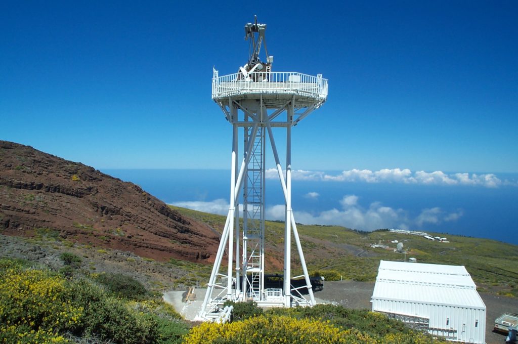
Dutch Open Telescope on La Palma, credits: astronomie.nl and Rob Hammerschlag.

Late 2003 and early 2004 I was a third year BSc student. I was lucky enough to be taken to La Palma by my professor Rob Rutten, presumably to use the Dutch Open Telescope, a fancy looking half alien with a 45 cm reflective telescope on top, that makes some awesome images (and movies!) of the solar atmosphere. It turned out to be cloudy for two weeks (on the mountaintop, lovely weather on the rest of beautiful island, not too bad….), so my “project” became more of a literature research and playing with some old data than an observational one.

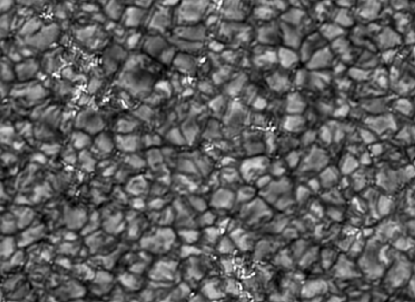
A tiny part of the solar surface — A small part of the surface of the Sun. The lighter areas are the top of convective cells where hot gas boils up. Cooling gas flows down in the darker lanes in between. The bright white points are places where the magnetic field of the Sun is strong and sticks through the surface.

I started looking into “bright points” in “intergranular lanes”. The granules, see left, are the top of convection cells, pretty much the upper layer of the boiling sun. In the darker lanes in between the cooling gas falls back down to be heated and boiled up and again later. Inside these darker lanes you sometimes see very bright spots. These are places where bundles of magnetic field stick up through the surface. These contain some less gas, so you look deeper into the Sun where it is hotter, hence the brightness of these spots.

With different filters you can choose at which height in the solar atmosphere you look (more or less; I guess you understand I take few shortcuts in my explanation here…), so we can see how such regions look higher up and see what the gas and these magnetic bundles do. Looking at a bundle from the top isn’t necessarily very informative, but when you look near the limb of the sun, you are basically getting a side view of these things:

Images near the limb of the Sun in three different filters taken simulateously. On the left you see a side view of the image above (on another part of the Sun at another time, though). Moving to the right are filters that typically see a little bit higher up in the atmosphere (the so-called chromosphere). For the interested reader: the filters are G-band, Ca II H and H-alpha. Image taken from Rutten et al. 2012.

I spent about 3 months discussing with the solar physics group in Utrecht, which still existed back in the day, trying to figure out how these magnetic fluxtubes actually work. I wrote a (admittedly mediocre quality) Bachelor’s thesis about this work that ends with some speculations. I fondly remember how my supervisor did not like my magnetic field structure based interpretation and believed it was more related to effects of the temperature structure and corresponding effect on how the radiation travels through these bits of atmosphere.

I suddenly was drawn back to this topic two weeks ago, when I read the Dutch popular astronomy magazine Zenit. It was a special about Minnaert’s famous “Natuurkunde van ‘t vrije veld” and featured an an article by the designer of the DOT, Rob Hammerschlag, and talked about observations of the Sun, including these magnetic structures. I followed some links from the article and found myself browsing the professional solar physics literature from the past decade or so, on the look for the current verdict on these “straws” in the middle image above.

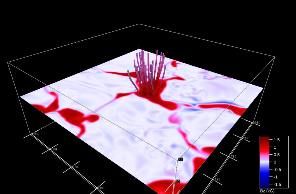
A detailed simulation of the solar surface and its magnetic field, by Chitta and Cameron from the MPS in Germany.

Obviously, the answer is slightly complicated and not as simple as mine (or my professor’s!) interpretation from 2004. While I was suggesting twisted magnetic field lines to be important, it turned out likely that the relevant phenomenon that is important in these straws are torsoidal waves through the tube (waves that you can make by grabbing it, and twisting like you twist the throttle of a motorcycle). Great fun to be taken back on a journey into the solar atmosphere, just by reading a simple popular article!

I regret quitting astrophysics

In 2013 I decided to quit my career in astrophysics, move back “home” and become a data scientist. The blog post I wrote about my decision was probably my best read publication as a professional astronomer and it was moving to read all the reactions from people who were struggling with similar decisions. I meant every word in that blog post and I still agree with most of what I said. Now, 7 years after the fact, it is time to confess: I deeply regret quitting.

This post is meant to give my point of view. Many people who left academia are very happy that they did. Here I present some arguments why one might not want to leave, which I hope will be of help for people facing decisions like these.

I miss being motivated. In the first few years after jumping ship many people asked me why I would ever wanted to not be a professional astronomer. I have always said that my day-to-day work wasn’t too different, except that what I did with data was about financial services or some other business I was in, rather than about galaxies and the Universe, but that the “core activities” of work were quite similar. That is kind of true. On an hour by hour basis, often I’m just writing (Python) code to figure things out or build a useful software product. The motivation to do what you do, though, is very very different. The duty cycle and technical depth of projects are short and shallow and the emphasis of projects is much more on getting working products than on understanding. I am doing quite well (in my own humble opinion), but it is hard to get satisfaction out of my current job.

I miss academic research. The seeds of astronomy were planted at very young age (8, if I remember correctly). The fascination for the wonders of the cosmos has changed somewhat in nature while growing up but hasn’t faded. Being at the forefront of figuring things out about the workings of the Universe is amazing, and unparalleled in any business setting. Having the freedom to pick up new techniques that may be useful for your research is something that happened to me only sporadically after the academic years. The freedom to learn and explore are valuable for creative and investigative minds and it doesn’t fit as well in most business settings that I have seen.

I miss working at academic institutions. The vibe of being at a large research institute, surrounded by people who are intrinsically motivated to do what they do was of great value to me. Having visitors over from around the globe with interesting, perhaps related work was a big motivator. That journal clubs, coffee discussions, lunch talks, colloquiums etc. are all “part of the job” is something that even most scientists don’t always seem to fully appreciate. Teaching, at the depth of university level classes, as a part of the job is greatly rewarding (I do teach nowadays!).

I miss passion and being proud of what I do. The internet says I have ”the sexiest job of the 21^st century”, but I think my previous job was more enjoyable to brag about at birthday parties. I can do astro as a hobby, but that simply doesn’t give you enough time to do something substantial enough.

I don’t miss … Indeed, the academic career also had its downsides. There is strong competition and people typically experience quite some pressure to achieve. The culture wasn’t always very healthy and diversity and equality are in bad shape in academia. Success criteria of your projects and of you as a person are typically better motivated in business. The obligatory nomadic lifestyle that you are bound to have as an early career scientist were a very enjoyable and educational experience, but it can easily become a burden on your personal life. The drawbacks and benefits of any career path will balance out differently for everybody. If you get to such a point, don’t take the decision lightly.

The people who questioned my decision to become an extronomer were right. I was wrong. It seems too late to get back in. I think I have gained skills and experience that can be very valuable to the astronomical community, but I know that that is simply not what candidates for academic positions are selected on. On top of that, being geographically bound doesn’t help. At least I will try to stay close to the field and who knows what might once cross my path.

Hacking for a future data flood

Astronomy has always been a “big data science”. Astronomy is an observational science: we just have to wait, watch, see and interpret what happens somewhere on the sky. We can’t control it, we can’t plan it, we can just observe in any kind of radiation imaginable and hope that we understand enough of the physics that governs the celestial objects to make sense of it. In recent years, more and more tools that are so very common in the world of data science have also penetrated the field of astrophysics. Where observational astronomy has largely been a hypothesis driven field, data driven “serendipitous” discoveries have become more commonplace in the last decade, and in fact entire surveys and instruments are now designed to be mostly effective through statistics, rather than through technology (even though it is still stat of the art!).

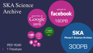
In order to illustrate how astronomy is leading the revolutions in data streams, this infographic was used by the organizers of a hackathon I went to nearing the end of April:
Streams and volumes of data!

The Square Kilometer Array will be a gigantic radio telescope that is going to result in a humongous 160 TB/s rate of data coming out of antennas. This needs to be managed and analysed on the fly somehow. At ASTRON a hackathon was organized to bring together a few dozen people from academia and industry to work on projects that can prepare astronomers for the immense data rates they will face in just a few years.

As usual, and for the better, smaller working groups split up and started working on different projects. Very different projects, in fact. Here, I will focus on the one I have worked on, but by searching for the right hash tag on twitter, I’m sure you can find info on many more of them!

We jumped on two large public data sets on galaxies and AGN (Active Galactic Nuclei: galaxies with a supermassive black hole in the center that is actively growing). One of them was a very large data set with millions of galaxies, but not very many properties of every galaxy (from SDSS), the other, out of which the coolest result (in my own, not very humble opinion) was distilled was from the ZFOURGE survey. In that data set, there are “only” just under 400k galaxies, but there were very many properties known, such as brightnesses through 39 filters, derived properties such as the total mass in stars in them, the rate at which stars were formed, as well as an indicator whether or not the galaxies have an active nucleus, as determined from their properties in X-rays, radio, or infrared.

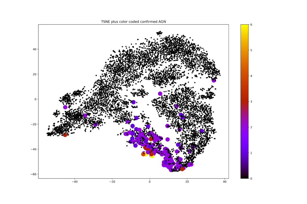
I decided to try something simple and take the full photometric set of columns, so the brightness of the objects in many many wavelengths as well as a measure of their distance to us into account and do some unsupervised machine learning on that data set. The data set had 45 dimensions, so an obvious first choice was to do some dimensionality reduction on it. I played with PCA and my favorite bit of magic: t-SNE. A dimensionality reduction algorithm like that is supposed to reveal if any substructure in the data is present. In short, it tends to conserve local structure and screw up global structure just enough to give a rather clear representation of any clumping in the original high dimensional data set, in two dimensions (or more, if you want, but two is easiest to visualize). I made this plot without putting in any knowledge about which galaxies are AGN, but colored the AGNs and made them a bit bigger, just to see where they would end up:
t-SNE representation of galaxy data from ZFOURGE

To me, it was absolutely astonishing to see how that simple first try came up with something that seems too good to be true. The AGN cluster within clumps that were identified without any knowledge of the galaxies having an active nucleus or not. Many galaxies in there are not classified as AGN. Is that because they were simply not observed at the right wavelengths? Or are they observed but would their flux be just below detectable levels? Are the few AGN far away from the rest possible mis-classifications? Enough questions to follow up!

On the fly, we needed to solve some pretty nasty problems in order to get to this point, and that’s exactly what makes these projects so much fun to do. In the data set, there were a lot of null values, no observed flux in some filters. This could either mean that the observatory that was supposed to measure that flux didn’t point in the direction of the objects (yet), or that there was no detected flux above the noise. Working with cells that have no number at all or only upper limits on the brightness in some of the features that were fed to the machine learning algorithm is something most ML models are not very good at. We made some simple approximations and informed guesses about what numbers to impute into the data set. Did that have any influence on the results? Likely! Hard to test though… For me, this has sprung a new investigation on how to deal with ML on data with upper or lower limits on some of the features. I might report on that some time in the future!

The hackathon was a huge success. It is a lot of fun to gather with people with a lot of different backgrounds to just sit together for two days and in fact get to useful results, and interesting questions for follow-up. Many of the projects had either some semi-finished product, or leads into interesting further investigation that wouldn’t fit in two days. All the data is available online and all code is uploaded to github. Open science for the win!

SAS in a Pythonista’s workflow

Most who know me will probably know that I’m a major fan of Python in particular and open source software in general. Still, in my day job I use SAS quite a lot. Because I will be at the SAS Global Forum in Denver next week, I thought it would be a good time to write about the place of SAS in my work.

First of all, I can obviously not pay for the massive license fees of software like SAS, which also is my biggest objection to using it. So when I do anything on a freelance basis, it will be purely Python, in almost all assignments. In my day job I arrived, now 4,5 years ago, in a team that even was called the “SAS team”. Their main, and in fact for a long time only, tooling was SAS Base. After fighting for a good two years we do now have a decent Anaconda installation with a Jupyter Hub which makes for much faster data exploration, easier analytics and easier and much prettier visualization (no, SAS Visual Analytics is *not* a visualization tool, it’s a dashboarding tool, enormous difference).

Alright, so I can use Python and R and I still use SAS? Indeed I do. I think every tool is good for something. Part of our team is mainly occupied with ETL (extract, transform, load) work, building a good, stable, clean and well structured data warehouse that others (like me) can use at ease. For such work, SAS has some great tools. Moving data from a data base that is designed to make a particular application work smoothly into a data warehouse, that keeps track of the history of that data base as well is not a trivial task and keeping track of all relevant input data base changes is quite some work. This is done with SAS (by others) and results in a data warehouse stored in SAS data sets that I consequently use for data analysis, machine learning, you name it.

From a data warehouse in SAS tables, I find it easiest to do my data collection, merging, aggregation and all that prerequisite work one always needs for analytics in SAS as well. Most of my projects start with data wrangling in SAS, and when I get to a small number of tables that are ready for analysis, analytics or visualization, I move over to Python (where the fun starts).

Yes, I do have my strong opinions about many SAS tools, about SAS as a company, about how they work and about how the world (e.g. auditors, authorities) look at SAS versus how they look at software from the open source realms. Still, I use a tool that is good at what I need from it, if I have access to it. More and better interfacing between Python, R and SAS is well underway and I hope the integration between the two will only become smoother. Hoping that SAS would vanish from my world is just an utterly unrealistic view of the world.

Why upgrade your OS if you don’t need to?

Two weeks ago I had nothing to do on a Saturday afternoon. Geeky as I am, I thought “let’s upgrade Xubuntu” on my laptop. I was still on the 16.04 Long Term Support version and it is 2018 by now, after all. A month or so later the new LTS version, 18.04, would appear, but why wait? That afternoon I had nothing better to do; when the new version comes out, I probably will be occupied. As usual, I googled around about a version upgrade from 16.04 to 17.10 and was, by every single site I encountered on the topic, strongly advised not to try this. But alas, I’m as stubborn as data scientists get and went ahead anyway.

Ouch. There seemed to be no problem at all. The upgrade was fine, except for some small weird looking error from LibreOffice, which I hardly ever use anyway. Everything worked as it worked before, even with the same looks (then why would you upgrade, right?). I played a game of Go for a bit and then went and let all other software do their updates as well. The usual reboot went blazing fast. I was prompted for my password and then the shit hit the fan: black screen. Nothing. Light from under the keyboard, but that was the only sign of life.

That is when you all of a sudden need a second computer. In all my confidence I had not created a bootable USB stick before the upgrade, and I didn’t have an older one with me either. With a terribly slow and annoying Windows laptop I managed to create one and booted the laptop from that. All fine. Good, so let’s replace the new and corrupted OS with something from this stick. Apparently, when I previously had installed my laptop, there seemed to be no need for a mount point for /efi, and now there was. Annoyingly, this needed to be at the start of the partition table, screwing up pre-existing partitions on that disk. At that point I decided: alright, format the disk, decently partition the disk and a fresh install would make my dear laptop all young and fresh again. There are two SSDs in the machine, and there was a back up of my home on the second disk.

The new install works like a charm, and restoring a back up also calls for some more cleaning up. It all looks tidy again.

I know, not everybody will be a fan of the old-school conky stuff on the desktop, but it just tickles my inner nerd a bit (and I actually do use it to monitor the performance when something heavy is running, I sure like it better than a top screen!). Took a decent part of a day, altogether, so next time I might take the advise of fellow geeks a bit more seriously. On the other hand, after mounting the second disk and finding the backups intact, the short moment of relief is worth it.

Off we go with a clean machine!

Craft beer!

One of my major interests outside the geeky realms is craft beer. I’m an avid sampler, try to go to beer festivals whenever I can, open Untappd almost every day, and I sometimes tweet about beer under a different twitter handle than my own: @BeerTweep.

In Dutch I have written (and hope to wrote again soon!) content for Bierista. You may be too lazy to go look on that site, so here’s a list of the specific things I wrote on there (newest first):

Fraude detecteren door vernuftige analyse

(This is a blog published on the website of my employer, thought it would make a fair placeholder, sorry about the Dutch).

De zorg is al duur zat. Elke extra euro die moet worden uitgegeven omdat een zorgverlener de regels buigt moet achterhaald, of liever nog voorkomen worden. Probleem is dat “die euro” dan wel gevonden moet worden en dat is geen sinecure. Dit komt door enerzijds het enorme volume aan declaraties dat een zorgverzekeraar krijgt van alle zorgverleners bij elkaar en anderzijds het feit dat fraudeurs slimme dingen bedenken om vooral niet op te vallen. Hoe sporen we bij DSW fraudeurs op?

Op zoek naar outliers

Naast de meer traditionele manieren om fraude op te sporen gebruiken we bij DSW ook analysetechnieken om in de grote bergen data die we hebben patronen te ontdekken die zouden kunnen wijzen op frauduleus of ander onwenselijk gedrag. De tandarts die in een jaar 20 vullingen legt bij een familielid of de psychiater die 40 uur per dag zegt te werken is natuurlijk gauw gevonden, maar de meeste boeven pakken het toch slimmer aan. Precies daarom moeten wij nog slimmer zijn!

Voor het detecteren van rotte appels in een fruitmand vol zorgverleners gaan we er over het algemeen van uit dat de grote meerderheid zich niet misdraagt. Dit betekent dat we kunnen zoeken naar zogenaamde “outliers”, personen of instanties die zich net even anders lijken te gedragen dan de norm. Een complicerende factor is dat wij als zorgverzekeraar altijd maar een deel van het gedrag van een zorgverlener kunnen controleren, namelijk alleen de zorg die gedeclareerd wordt voor die patiënten die toevallig bij ons verzekerd zijn. Bij sommige instanties is dat misschien wel 60% van de populatie of meer, maar bij de meesten toch duidelijk minder, en we weten niet eens hoeveel precies. We hebben dus eerst wat werk te verzetten om analyses te doen op grootheden die niet zo gevoelig zijn voor het marktaandeel van DSW, zoals bijvoorbeeld kosten per verzekerde.

De score opbouwen

Alleen controleren op een getal als de gemiddelde kosten per verzekerde dekt de lading ook niet. Als een kwaadwillende zorgverlener dan kleine bedragen declareert voor een hoop mensen, dan gaat hij zelfs lager eindigen in kosten per verzekerde (terwijl hij in het aantal mensen waarvoor iets declareert juist weer zou opvallen). We kijken daarom naar heel veel van dit soort graadmeters tegelijk. Zo bouwen we een “score” op die aangeeft op hoeveel van dit soort anomaliedetecties (en andere controles) een zorgverlener opvalt, en hoe sterk hij opvalt.

Naast het detecteren van grootheden waarop een zorgverlener opvalt door ander gedrag dan zijn/haar concurrenten, kunnen we ook kijken naar signalen van verzekerden (“ik heb die behandeling helemaal niet gehad”), naar simpele regels als “geamputeerde ledematen kun je niet meer breken” of zelfs naar (zakelijke) verbanden tussen verschillende zorgverleners waardoor lucratieve doch frauduleuze werkwijzen kunnen worden overgebracht van de doorgewinterde oplichter naar de crimineel in spe.

Verder onderzoek

Alle ingrediënten van een totaalscore zijn hard te maken met statistiek, wet- en regelgeving of andere afspraken. Door het tweaken van de opbouw van zo’n totaalscore maken we een lijst waarvan we toch met enige zekerheid wel kunnen zeggen dat er iets loos is. Wanneer dergelijke signalen zijn gegenereerd dan pakken andere afdelingen dit doorgaans op voor verder onderzoek. Hiervoor levert ons datateam uiteraard nog wel data en analyses aan, maar het initiatief voor het uiteindelijk aanpakken ligt dan in de handen van de afdelingen die dichter bij de dagelijkse gang van zaken van een zorgverlener staan.