I was already convinced years ago, by videos and a series of blog posts by Jake VanderPlas (links below), that if you do inference, you do it the bayesian way. What am I talking about? Here is a simple example: we have a data set with x and y values and are interested in their linear relationship: y = a x + b. The numbers a and b will tell us something we’re interested in, so we want to learn their values from our data set. This is called inference. This linear relationship is a model, often a simplification of reality.
The way to do this you learn in (most) school(s) is to make a Maximum Likelihood estimate, for example through Ordinary Least Squares. That is a frequentist method, which means that probabilities are interpreted as the limit of the relative frequencies for very many trials. Confidence intervals are the intervals that describe where the data would lie after many repetitions of the experiment, given your model.
In practice, your data is what it is, and you’re unlikely to repeat your experiment many times. What you are after is an interpretation of probability that describes the belief you have in your model and its parameters. That is exactly what Bayesian statistics gives you: the probability of your model, given your data.
For basically all situations in science and data science, the Bayesian interpretation of probability is what suits your needs.
What, in practice, is the difference between the two? All of this is based on Bayes’ theorem, which is a pretty basic theorem following from conditional probability. Without all the interpretation business, it is a very basic result, that no one doubts and about which there is no discussion. Here it is:
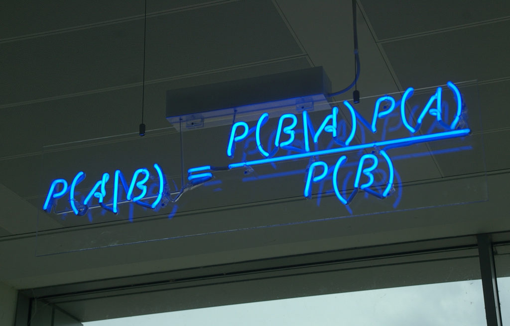
Now replace A by “my model (parameters)” and B by “the data” and the difference between inference in the frequentist vs Bayesian way shines through. The Maximum Likelihood estimates P(data | model), while the bayesian posterior (the left side of the equation) estimates P (model | data), which arguably is what you should be after.
As is obvious, the term that makes the difference is P(A) / P(B), which is where the magic happens. The probability of the model is hat is called the prior: stuff we knew about our model (parameters) before our data came in. In a sense, we knew something about the model parameters (even if we knew very very little) and update that knowledge with our data, using the likelihood P(B|A). The normalizing factor P(data) is a constant for your data set and for now we will just say that it normalizes the likelihood and the prior to result in a proper probability density function for the posterior.
The posterior describes the belief in our model, after updating prior knowledge with new data.
The likelihood is often a fairly tractable analytical function and finding it’s maximum can either be done analytically or numerically. The posterior, being a combination of the likelihood and the prior distribution functions can quickly become a very complicated function that you don’t even know the functional form of. Therefore, we need to rely on numerical sampling methods to fully specify the posterior probability density (i.e. to get a description of how well we can constrain our model parameters with our data): We sample from the priors, calculate the likelihood for those model parameters and as such estimate the posterior for that set of model parameters. Then we pick a new point in the priors for our model parameters, calculate the likelihood and then the posterior again and see if that gets us in the right direction (higher posterior probability). We might discard the new choice as well. We keep on sampling, in what is called Markov Chain Monte Carlo process in order to fully sample the posterior probability density function.

On my github, there is a notebook showing how to do a simple linear regression the Bayesian way, using PyMC3. I also compare it to the frequentist methods with stasmodels and scikit-learn. Even in this simple example, a nice advantage of getting the full posterior probability density shines: there is an anti-correlation between the values for slope and intercept that makes perfect sense, but only shows up when you actually have the joint posterior probability density function:


Admittedly, there is extra work to do, for a simple example like this. Things get better, though, for examples that are not easy to calculate. With the exact same machinery, we can attack virtually any inference problem! Let’s extend the example slightly, like in my second bayesian fit notebook: An ever so slightly more tricky example, even with plain vanilla PyMC3. With the tiniest hack it works like a charm, even though the likelihood we use isn’t even incorporated in PyMC3 (which makes it quite advanced already, actually), we can very easily construct it. Once you get through the overhead that seems killing for simple examples, generalizing to much harder problems becomes almost trivial!
I hope you’re convinced, too. I hope you found the notebooks instructive and helpful. If you are giving it a try and get stuck: reach out! Good luck and enjoy!
A great set of references in “literature”, at least that I like are:
- A blog series by Jake VanderPlas.
- A nice PyMC3 tutorial by BDFL Chris Fonnesbeck.
- A fun podcast: Learning Bayesian Statistics by Alex Andorra (if not only for the soundtrack….).
- The official PyMC3 tutorials.
- Bayesian Methods for Hackers by Cameron Davidson-Pilon (PyMC3 version).